Why Random Shuffling improves Generalizability of Neural Nets

You must have both heard and observed that randomly shuffling your data improves a neural network's performance and its generalization capabilities. But what is the possible reason behind this phenomenon? How can just shuffling data provide performance gains? Well, let's find out!

A Simple Thought Experiment

Let's say that you are working on a problem that requires a deep learning based solution and assume that you already built the required network architecture. This architecture is composed of multiple weights which are nothing but floating point numbers.

Now, imagine a square which is completely filled with dots with only a single dot being highlighted. This special dot represents your model with its randomly initialized current weights. Any change, whatsoever, in the model's weights will result in a different dot being highlighted. Thus, each dot represents a possible state for your model and the square is the entire state space a.k.a. search space (see Fig. 1). One of the dots in this space represents the model with optimal weights which is equivalent to hitting the global optima. The goal of any gradient descent algorithm such as Stochastic Gradient Descent (SGD) or ADAptive Moment estimation (ADAM) is to traverse the search space in order to find this "dot". The further away you start from this goal, the harder it is going to be for your model to reach the global optima due to "hurdles" (local optimas) in the path. This is why the deep learning community stresses on better weight initialization schemes.

From any gradient descent algorithm, we know that the parameters (weights) of a model are updated based on gradients. In other terms, gradients guide the traversal of the search space.

Coming back to our experiment, let us assume that we have 10 batches of data to train our model. Each batch provides us with corresponding gradients for updating the model's parameters. For simplicity, let us assume that the gradients from each batch traverses the search space in one of the four directions (left, top, right, bottom). This means that everytime we update the model parameters with the gradient of a single batch, a new dot, which is either the first dot to the left, top, right or bottom of the current dot, is highlighted in the search space .

Fig. 1: A visual representation of the thought experiment. Without shuffling the data leads to network parameter updates with states that are in an overall similar direction

If we do not shuffle the data, then the order of the batches remains the same. Even though each gradient update highlights a different dot in a different direction, the overall direction of updation remains the same. What this means is that if in the first epoch, the overall direction in which new dots are being highlighted is, say, top left (north-west), then this direction will remain the same in the next epoch because the order of the gradient updates have not changed (see Fig. 1).

Fig. 2: Shuffling the data leads to network parameter updates with states that are in an overall different direction. This allows for the traversal of a larger subset of the search space

But why is this a problem? Its because traversing the search space in a single direction is restricting the possible states that our model could achieve. This reduces the probability of finding the global optima or in other words, the optimal state for our model. Without shuffling we are in effect searching through only a subset of the entire state/search space. As you can understand, this is not necessarily bad because there is still a small probability that, by chance, the direction we are traversing in might actually lead to us to the global optima. This is why, sometimes, we achieve better scores on the test set without shuffling. But such a probability is very low which is why most often than not, shuffling data provides superior results.

Proof Through Code

Enough talk. Let's prove our hypothesis with actual code and visualization.

Task: Train a model on a dataset and check how the value of the weights in the network change at every epoch. Since change in weights are directly related to gradients, we therefore check the gradient values for each batch at every epoch. Based on the simple thought experiment, our hypothesis is that without shuffling, the gradients for each batch at every epoch should point in a similar direction. Thus, we should expect a smooth plot while with shuffling, the gradient directions should change abruptly. Therefore, we should expect a rough plot.

As you know, gradients are high-dimensional vectors where each dimension is the number of weights. Thus, we went with the UrbanGB dataset from UCI repository as it has only two features which will help us in visualizing on the 2D plane. The dataset consists of 3,60,177 examples, so we randomly sample 10,000 examples for this experiment.

Code to pre-process and get our training data in NN digestible format

As per Fig. 3, we have two neurons for input, $X1$ and $X2$, since there are two features in the dataset; one neuron, $Z1$ in the hidden layer and 461 neurons in the output layer. We choose only a single neuron in the hidden layer as it gives us two weights, $W1$ and $W2$, that we can easily visualize on a 2D plane. The output has 461 neurons as that many classes exist in the target variable.

Fig. 3: The network architecture used for the experiment

We divide the data into 10 batches of 1000 samples each. We will focus on the gradients of each batch at every epoch for the weights $W1$ and $W2$ only. The number of epochs for training is set to 10. Only a small number of epochs is used as the goal of this experiment is not to achieve high accuracy but to prove our hypothesis.

Code for building and training the model. Gradients for the weights are stored for each batch at every epoch

It is clear from Fig. 4, that without shuffling, the gradients of each batch change smoothly over multiple epochs denoting that they traverse an overall similar direction which is also visible in the plot itself ($W1$ gradients moving towards the bottom while $W2$ gradients moving towards the top). While, with shuffling, the gradients are all over the place with no specific overall direction which denotes that more states are being searched in order to find the global optima. This also goes on to show why some gradient descent algorithms such as SGD have noisy loss plots when shuffling is switched on.

(a)

(c)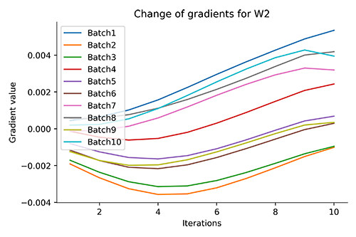

(b)

(d)

Fig. 4: (a) & (b) Without Shuffling - For each batch, we get to see the overall change in direction of the gradients for W1 and W2, respectively, at every epoch
(c) & (d) With Shuffling - For each batch, we get to see the overall change in direction of the gradients for W1 and W2, respectively, at every epoch

Conclusion

There are multiple ways to explain why shuffling improves generalization in neural networks including the following brilliant answer on StackExchange. We believe this article to be an intuitive method for understanding this topic as it allows us to explain a few more phenomena and observations along the way. Your main takeaway should be that, most observations related to a neural network can be explained through gradients as it is the only quantity which updates your network parameters.